The Lorenz Butterfly

The Lorenz System

The Lorenz system is a (vector-valued) ordinary differential equation studied by the eponymous Edward Lorenz. It is most simply stated as a first-order ordinary differential equation for three functions: $x(t), y(t), z(t)$. These three functions satisfy the following differential equation.

Here, σ, ρ, and β are (real) constants. The behavior of the Lorenz system over time depends on these three constants. Given any initial point $(x, y, z)$, this system can be evolved over time, tracing out a curve in three-dimensional space. In the curve that is shown below, we take

In this figures, we start with the initial point $(x, y, z) = (1,0,0)$. For reference, a white dot is placed at $(0,0,0)$. The interesting feature of the Lorenz system is that it usually exhibits chaotic behavior. This means that the behavior is, in a sense, unpredictable. A small change in the initial point leads to a large change in the final trajectory after a surprisingly short span of time. Many systems in life, and especially physics, can be modeled by differential equations. The most well-studied of these differential equations are easy to study, and hence non-chaotic. However, a ton of natural systems display chaotic behavior such as the weather, turbulent fluid flow, the double pendulum, and a whole lot more. The chaotic nature of weather systems is one reason why it is so hard to get accurate weather predictions: any small uncertainty in the initial weather conditions becomes a huge uncertainty in the weather conditions a week later. The study of these chaotic systems has been coined "chaos theory".

Solving the Lorenz system

To play the simulation of the Lorenz attractor, press the start button below, or press p. Zoom in/out with a scroll wheel, or with the keys + and -. Rotate the image by using the arrow keys, or WASDQE keys. Watch and enjoy!

In case you did't want to wait for the above simulation to play out, you can find a screenshot of how it looks after a long time below. The color of the path is set to change over time, so you can observe which parts of the figure were drawn at which time. This pattern is traced out over and over again, although never in exactly the same way. Theoretically, the pointer never returns to the same place twice, yet it will always trace out these two lobes.

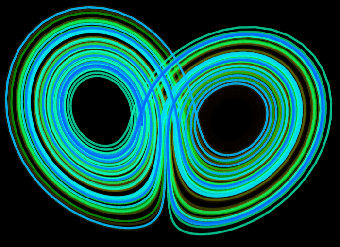
Looks cool, right? This shape is called the Lorenz butterfly. I think it is mesmerizing to watch the pointer trace out such a beautiful pattern from, really, such a simple equation. The solution appears to randomly jump from one half of the butterfly to the other, without warning, tracing out a new ring for the "wing" of the butterfly. This unpredictability in the trajectory of a solution to the Lorenz system is due to its chaotic behavior.

Chaos Theory

To fully appreciate the chaotic nature, it pays to look at how two close, but different, paths change over time. In what is called a stable solution, these two paths would converge to each other, so that small differences in the initial position become undetectable after a long time. The Lorenz system is definitely not stable. In the next simulation, I put two different solutions to the system with different initial points. I've also decreased the tail length so that the relationship between these two solutions is clearer. Notice how the two solutions begin close together but soon separate. After they separate, they appear to become completely uncorrelated, so that there it is impossible to predict where one solution will be based on the other.

It's slightly hypnotic, watching these curves trace out seemingly random curves through space, but knowing that it is all completely determined by the exact initial conditions. This is actually one of the reasons why weather is so hard to predict: the defining differential equations of weather are chaotic, so any uncertainty in intial weather conditions compounds over time into large uncertainty in the final weather. And it is impossible to measure weather conditions precisely. So, setting apart the (separate) issue of differential equations like weather (and more generally, PDEs) being hard to model, it is impossible to predict the weather too far into the future. Some meteorologists predict that we will never be able to accurately model more than two weeks in the future because of this (source). The phenomenon of chaos is also sometimes called the "butterfly effect" because, as the warning goes, the difference between clear skies and a hurricane may start with something as small as the flap of a butterfly's wing.

Okay, I have a confession. This isn't really the solution to the Lorenz system. The truth is that just as small errors in the initial position can compound to produce very different trajectories, so can small errors when solving the differential equation. Although the exact solution traces out the same butterfly shape, its trajectory will be different.

The simplest way to solve a differential equation is using Euler's Method. I won't discuss the details here, but Wikipedia has a great explanation (with code) for those who are interested. If you want to write a quick differential equation solver that gets the job done, this is your simplest choice. However, it is not always accurate enough, so mathematicians throughout the centuries have come up with countless numerical techniques that improve on Euler's method. The most famous of these is, perhaps, the 4th Order Runge-Kutta Method often just called the Runge-Kutta Method. This is the method that I have been using to draw pretty butterflies, but even it is not perfect. Chaotic systems are great at amplifying the effect of small errors, and we will use the Lorenz system to picture the difference between the Runge-Kutta and Euler methods.

In the following simulation, we use vibrant blue to represent a solution with Euler's method and vibrant green to represent a solution with the Runge-Kutta Method. I have also included solutions with both methods that are twice as accurate, given by dull blue and dull green respectively. (Technically, the dull solutions have half the step size). All four trajectories begin with the same initial conditions. The Euler's Method (blue) solutions immediately diverge because the Euler method is less accurate. The Runge-Kutta (green) solutions stay together for a while, but they too eventually diverge.

If you've stayed with me this far, I hope you have learned to see the beauty in differential equations, and especially in chaos. The Lorenz Butterfly is only the tip of the iceberg: it is just one example of a so-called strange attractor, a fractal-like shape traced out by a differential equation. Other strange attractors include the Rössler Attractor and Chua's Attractor.

The idea of chaos transcends even differential equations. Many (discrete) sequences can exhibit chaotic behavior such as the Logistic Map. For those interested in mathematics, pretty pictures, or the unpredictable nature of life, I recommend learning more about chaos.

Lastly, I can't leave without giving you one last simulation. Because I think it's beautiful, here is the Lorenz Butterfly traced out by ten different solutions with slightly different initial conditions. For better effect, I have increased the speed with which the solutions change color. After 30 seconds or so, I find that I have already lost track of which solution began as which!

I hope you enjoy!